For a commutative ring 


For idempotent 


Complementary idempotents give a formulation of an inner product. What do I mean by this? If 


What do idempotents of some rings look like? 

What about rings 


We can now look at the general case, let 


 be
be  distinct complex numbers and let
  be
be  such that
  for
for  ?
? satisfying the above! This polynomial is called the Lagrange interpolation polynomial and is constructed explicitly.
 and let
  .
. is a polynomial of degree
  with
with  and
and  if
if  .
. is another polnomial of degree
  for
for  , and takes
  . This polynomial picks out an idividual point and ignores all the rest, this is precicely what we need.
 which is a polynomial of degree
  with the properties we want.
 , the difference
  vanishes at
  and hence
  .
. where
where  for
for  and
and  . The atypical example is a matrix algebra of dimension
  denoted
  . There is a notion of algebra morphism which is not too hard to figure out with the above or a quick google, so we have a notion of isomorphism.
 where
where  . As a collection, they are denoted
  . These form a vector space and as algebras
  . Where the algebra operation in
  is matrix multiplication and
  is the algebra of vector space automorphisms
  with the algebra operation being composition.
 to a general
  -modules? These are in fact abelian groups (why?) and so the collection of possible ‘vectors’ for
  on the space, this pair is called a topological vector space when
  is closed for all
  and both vector space operations are continuous. This being addition and scalar multiplication.
 by
by  where
where  it’s not hard to show that
  is in fact a homeomorphism. This gives us that the topology is uniquely defined local, around some point say
  because
  is open iff
  is open for all
  a young mathematician will learn the inequality
  which has its name associated to Cauchy and Schwarz and is called the Cauchy -Schwarz inequality.
 for some
  and for all
  . Here is a neat niave proof of this result following the mathematicians’ philosophy of ‘look for symmetry’.

 Yes I did just write this and no, I’m not insulting your inteligence. This is my apeal to symmetry.
 I’ll let you finish the rest off but we’ve done all the hard work here.
 . Given a sequence
  where
where  we have a collection of partial sums
  indexed by
  and defined by
  . If the sequence
  converges to
  (In the usual
  –
– way) we say the series converges and write
  . For completness if the sequence
  and
and  for
for  ). In particular the
  are real numbers. Then the series
  converges if and only if the series
  converges.
 and
and  . We will look at two cases, when
  and when
  .
. where the first inequality followed from
 where the first inequality follows from
  are either BOTH bounded or BOTH unbounded which completes the proof.
 that
that  converges if
  and diverges if
  .
. increases which puts us in good position to apply our theorem. This leads us to the following which is enough as a proof.
 .
. be a finite group and
  a prime such that the order of
  where
where  are coprime.
  whose order is
  we have the order of
  dividing the order of
  or a cyclic group
  . As our goal (sorry I didn’t tell you this earlier) is to look at the subgroups of
  where
where  .
. and
and  is prime the result follows from Cauchy’s Theorem. Now suppose we can always find a
 ![|G| = |H|[G:H]](https://s0.wp.com/latex.php?latex=%7CG%7C+%3D+%7CH%7C%5BG%3AH%5D+&bg=ffffff&fg=404040&s=0&c=20201002) so if
so if ![[G:H]](https://s0.wp.com/latex.php?latex=%5BG%3AH%5D&bg=ffffff&fg=404040&s=0&c=20201002) we can apply the inductive hypothesis to
we can apply the inductive hypothesis to ![[G:H]](https://s0.wp.com/latex.php?latex=%5BG%3AH%5D+&bg=ffffff&fg=404040&s=0&c=20201002) is divisible by
is divisible by  where
where  . Applying the orbit stabiliser theorem tells us for each orbit
  we have
 ![|G * x| = [G:G_x]](https://s0.wp.com/latex.php?latex=%7CG+%2A+x%7C+%3D+%5BG%3AG_x%5D&bg=ffffff&fg=404040&s=0&c=20201002) where
where  is its stabiliser. Orbits partition
 ![|G| = |Z(G)| + \sum [G:G_x]](https://s0.wp.com/latex.php?latex=%7CG%7C+%3D+%7CZ%28G%29%7C+%2B+%5Csum+%5BG%3AG_x%5D+&bg=ffffff&fg=404040&s=0&c=20201002) where
where  is the abelian subgroup
  of G which is often called the center of
  and applying Cauchy’s Theorem we can find an element
  of order
  we have
  .
. and a quotient map
  and applying the inductive hypothesis to
  gives us a
  due to the equality
  from Lagrange. Looking at
  as
as  and
and  maps
maps  into
into  we have
  and applying Lagrange (again) we obtain
  , as desired. We have found our
  anymore. But you want to keep doing analysis.
 . Note that this inequality does not hold under our usual absolute value, for example:
  . But does this tweaking of the triangle inequality add anything new? It may not look like it at first, but it is a dream come true: a sequence is Cauchy if and only if distance of consecutive terms goes to zero! More mathematically: the sequence
  is Cauchy
 as
as 
 is not Cauchy in the reals
  which clearly tends to zero.
 however this would work in any metric space
  where the triangle inequality satisfies
  for any
  . This is because an absolute value on
  .
. be an absolute value on
  . Then any sequence
  Let
Let  . Since
  such that for all
  we have
  . In particular, whenever
  , we obtain
 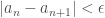 , which means that
  as
as  Let
Let  .
. , applying our strict triangle inequality:
 .
.

 is the exponent of
  whenever we write the rational number as
  , where
  are coprime to
 ![K[x_1,...,x_n]](https://s0.wp.com/latex.php?latex=K%5Bx_1%2C...%2Cx_n%5D+&bg=ffffff&fg=404040&s=0&c=20201002) be the commutative polynomial ring with
be the commutative polynomial ring with  variables (if you are familiar with this ring I would skip the next paragraph)
![K[x_1,...,x_n]](https://s0.wp.com/latex.php?latex=K%5Bx_1%2C...%2Cx_n%5D&bg=ffffff&fg=404040&s=0&c=20201002) look like? Taking
look like? Taking  it is not hard to come up with elements, for example
  . One can quite easily start conjuring up polynomials for a given
  . We can simplify the notation by starting with an
  of non-negative integers and letting
  . Clearly a poynomial
 ![f \in K[x_1,...,x_n]](https://s0.wp.com/latex.php?latex=f+%5Cin+K%5Bx_1%2C...%2Cx_n%5D&bg=ffffff&fg=404040&s=0&c=20201002) can be written as a finite linear combination of moninomials with the general form
can be written as a finite linear combination of moninomials with the general form  where
where  and
and  with
with  also being finite. Without knowing what a polynomial is aprior this is the method used to define what a polynomial is with
 ![f \in K[x_1,...,x_n]](https://s0.wp.com/latex.php?latex=f+%5Cin+K%5Bx_1%2C...%2Cx_n%5D+&bg=ffffff&fg=404040&s=0&c=20201002) we can think of it as an algebraic element of our ring or a function
we can think of it as an algebraic element of our ring or a function  by swapping
  with some
  for all
  . This gives us two notions of zero; the zero element of
  .
. ,
,  and look at the polynomials
  and
and  in
in ![K[x]](https://s0.wp.com/latex.php?latex=K%5Bx%5D&bg=ffffff&fg=404040&s=0&c=20201002) . As algebraic elements clearly
. As algebraic elements clearly  is the zero element and
  isn’t but as functions
  and
and  so we can conclude both
  .
. .
. by Lagrange’s Theorem and looking at the multiplicative group
  one can show
  for all
  so the polynomial
  is a zero function but is distinct from the zero element in
  . This tells us that when
  if and only if
  is the zero function.
![f = 0 \in K[x_1,...,x_n]](https://s0.wp.com/latex.php?latex=f+%3D+0+%5Cin+K%5Bx_1%2C...%2Cx_n%5D+&bg=ffffff&fg=404040&s=0&c=20201002) trivially we must have
trivially we must have  for all
  . The other direction requires us to show that if for some
  is the zero element in
  a non-zero polynomial in
 ![K[x]](https://s0.wp.com/latex.php?latex=K%5Bx%5D+&bg=ffffff&fg=404040&s=0&c=20201002) of degree
of degree  has at most
 ![f \in K[x]](https://s0.wp.com/latex.php?latex=f+%5Cin+K%5Bx%5D+&bg=ffffff&fg=404040&s=0&c=20201002) such that
such that  and since
  let
let  for all
  we can write
  where
where  is the highest power of
  that appears in
 ![g_i \in K[x_1,...,x_{n-1} ]](https://s0.wp.com/latex.php?latex=g_i+%5Cin+K%5Bx_1%2C...%2Cx_%7Bn-1%7D+%5D+&bg=ffffff&fg=404040&s=0&c=20201002) . If we show that
. If we show that  is the zero polynomial in
  we get a polynomial
 ![f(\alpha_1,...,\alpha_{n-1}, x_n) \in K[x_n]](https://s0.wp.com/latex.php?latex=f%28%5Calpha_1%2C...%2C%5Calpha_%7Bn-1%7D%2C+x_n%29+%5Cin+K%5Bx_n%5D+&bg=ffffff&fg=404040&s=0&c=20201002) and by our hypothesis this polynomial vanishes for all
and by our hypothesis this polynomial vanishes for all  . Using our above representation of
  are
are  and hence
  for all
  and so by the inductive hypothesis
 ![K[x_1,..., x_n]](https://s0.wp.com/latex.php?latex=K%5Bx_1%2C...%2C+x_n%5D+&bg=ffffff&fg=404040&s=0&c=20201002) .
.![f ,g \in K[x_1,...,x_n]](https://s0.wp.com/latex.php?latex=f+%2Cg+%5Cin+K%5Bx_1%2C...%2Cx_n%5D&bg=ffffff&fg=404040&s=0&c=20201002)
 in
in  and
and  are the same functions. I leave the proof of this for the reader and as a hint consider the polynomial
  .
. which is a famous result pioneered by the work of
 ![p \in \mathbb{R}[x]](https://s0.wp.com/latex.php?latex=p+%5Cin+%5Cmathbb%7BR%7D%5Bx%5D+&bg=ffffff&fg=404040&s=0&c=20201002) be a polynomial over
be a polynomial over  where
where  and that
  for all
  and some
  . We will be considering our polynomial as a function
  and be setting
  and
and  where our choice of
  will be more apparent later.
 of a large enough magnitude our polynomial will have a magnitude as large as we like. We will also establish a simple bound on the magnitude of the roots of our polynomial
  , we have
  by the definition of our constants and estimating
  gives
gives  by using the sum of a geometric series and the triangle inequality.
 which gives us by using the previous estimation
  as both
  and
and  as
as  .
. we have
  .
. for some
  and
and  or equivalently
  . If we take
  we have that
  giving us a bound on the size of our root in terms of the polynomials coefficients. This means all roots of
  .
.